Lecturer: Ph.D., Associate Professor Bosak Alla Vasylivna
The purpose of studying the discipline is to form in students the theoretical knowledge and practical skills of using the most modern integrated systems of computer mathematics in solving mathematical problems of different classes. The study of the material of this discipline is focused on the widespread use of computer technology and programming.
The subject of the discipline is integrated computer mathematics systems.
The result of studying the discipline is the formation of students’ abilities:
- use modern methods of computer mathematics systems to solve engineering problems in the field of power engineering, electrical engineering and electromechanics;
- create and apply algorithms to solve typical problems;
- solve basic symbolic and numerical problems, construct graphs of functions, solve linear and nonlinear equations, use numerical integration and solution of differential equations of different classes.
The discipline “Integrated systems of computer mathematics” consists of 3 sections:
- Section 1. Introduction to the discipline “Integrated systems of computer mathematics”:
Topic 1.1. Review and comparative analysis of basic computer mathematics systems.
Topic 1.2. Use of structural and object-oriented programming by means of ISKM - Section 2. MathCAD integrated system:
Topic 2.1. Consideration of the main properties of the software package MathCAD. Automated design systems. System user interface.
Topic 2.2. Calculation of results of mathematical operations. Numeric constants, variables, functions, etc. Operations with vectors and matrices.
Topic 2.3. Plotting graphs of functions.
Topic 2.4. Using the MathCAD system to solve nonlinear equations. Numerical integration.
Topic 2.5. Approximation of functions. Solving systems of differential equations. Systems with variable parameters. - Section 3. MATLAB integrated system:
Topic 3.1. MATLAB system. The main components of the user interface. Interactive environment. Getting started with the system.
Topic 3.2. Mathematical calculations. Creating algorithms. Working area of the environment. Graphic capabilities of the system. Construction of function graphs.
Topic 3.3. Using the Matlab system to solve nonlinear equations. Numerical integration. Using the Matlab system to solve differential equations.
Topic 3.4. Environment expansion packages. SIMULINK. TOOLBOXES. The main purpose of mathematical packages. Areas of application. Using special methods to work with the environment.
Basic literature:
- Lozynsky AO Solving problems of electromechanics in the environments of MathCAD and MATLAB packages / AO Lozynsky Lozynsky, VI Moroz, Ya.S. Paranchuk: Textbook. – Lviv: Lviv Polytechnic State University Publishing House, 2000. – 166 p.
- Lavrentik AI MathCAD. Lecture notes / AI Лаврентик, О.А. Tuzenko: Mariupol: PSTU, 2010. – 114 p.
- Information technologies: Systems of computer mathematics [Electronic resource]: textbook. way. for students. specialties “Automation and computer-integrated technologies” / IV Kravchenko, VI Mykytenko; KPI them. Igor Sikorsky. – Electronic text data (1 file: 5.57 MB). – Kyiv: KPI named after Igor Sikorsky, 2018. – 243p.
- Revinskaya OG R32 Fundamentals of programming in MatLab: textbook. allowance. – СПб .: БХВ-Петербург, 2016. – 208 с.
- Мирановский Л.А. Introduction to MATLAB: Textbook. manual / LA Mironovsky, K. Yu. Petrova; GUAP. – СПб., 2006. – 164 с.
Supporting literature:
- Govorukhin V., Tsibulin V. Computer in mathematical research. Training course. – СПб .: Питер, 2001. – 624 с .: ил.
- Dyakonov VP Mathematical system Maple V R3 / R4 / R5. – M .: “SO-LON”, 1998.
- Plis AI, Slivina NA Mathcad: mathematical workshop. – Moscow: Finance and Statistics. –1999.
- Dyakonov VP, Abramenkova IV MathCAD 7 in Mathematics, Physics and the Internet. – М: Нолидж, 1998. – 352 с.
Information resources
http: // uk.wikipedia.org – Website of the world-famous electronic encyclopedia
http://www.exponenta.ru – Educational mathematical website
http://planetmath.org – Website of the world mathematical encyclopedia
http: / /allmatematika.ru – Mathematical forum
http://www.forum.softweb.ru – Web-page of the forum of mathematical and engineering software
http://model.exponenta.ru – Web-site of modeling of systems and phenomena
Link to Moodle: https://do.ipo.kpi.ua/course/view.php?id=511
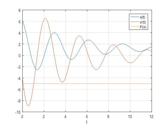
Solving the second-order differential equation with a special nonlinear part using Matlab:
function du = diffsys (t, u); %
declaration of the function for the solution of the system global a1 a2% declaration of constants
% explanation
% u (1) -> x (t)
% u (2) -> dx / dt
% du (1) -> dx / dt
% du (2) -> d2x / td2
% system in Cauchy form:
d2x / dt2 = -F (x) – a1 dx / dt – a2 x; % record of the right part of the system
du = zeros (2,1); % blank from zeros
du (1) = u (2);
du (2) = -F (u (1)) – a1 u (2) -a2 u (1);
function y = F (x)
global M2 l1 l2 f1; % declaration of constants
y = zeros (size (x)); % blank from zeros
for i = 1: numel (x)
if x (i) <0
y (i) = -M2;
elseif x (i) <= l2
y (i) = 0;
elseif x (i) <l1
y (i) = (x (i) -l2) / (l1-l2) * f1;
else
y (i) = f1;
end
end
global a1 a2 M2 l1 l2 f1% declaration of constants
% values of variables:
a1 = 1;
a2 = 0.1;
M2 = 10;
l1 = 0.4;
l2 = 0.2;
f1 = 50;
% time range:
tk = [0, 8];
% initial conditions:
x0 = [-6, 4];% x (0), x` (0)
% we solve:
[TX] = ode45 (‘diffsys’, tk, x0);
plot (T, X, T, F (X (:, 1)))% graph output
grid on%
legend (‘x (t)’, ‘x ”(t)’, ‘F (x)’)% signature
xlabel curves (‘t’)